mplotqueries#

mplotqueries is a tool to visualize operations in MongoDB log files. It has several different plot types and can group information in various ways.

NOTE: logv2 format (MongoDB 4.4+) is not supported yet.

Usage#

mplotqueries [-h] [--version] logfile [logfile ...]
             [--group GROUP]
             [--logscale]
             [--type {nscanned/n,rsstate,connchurn,durline,histogram,range,scatter,event} ]
             [--overlay [ {add,list,reset} ]]
             [additional plot type parameters]
             [--dns]
             [--checkpoints]
             [--oplog]

mplotqueries can also be used with shell pipe syntax, for example:

mlogfilter logfile [parameters] | mplotqueries --type histogram

General Parameters#

Help#

-h, --help: shows the help text and exits.

Version#

--version: shows the version number and exits.

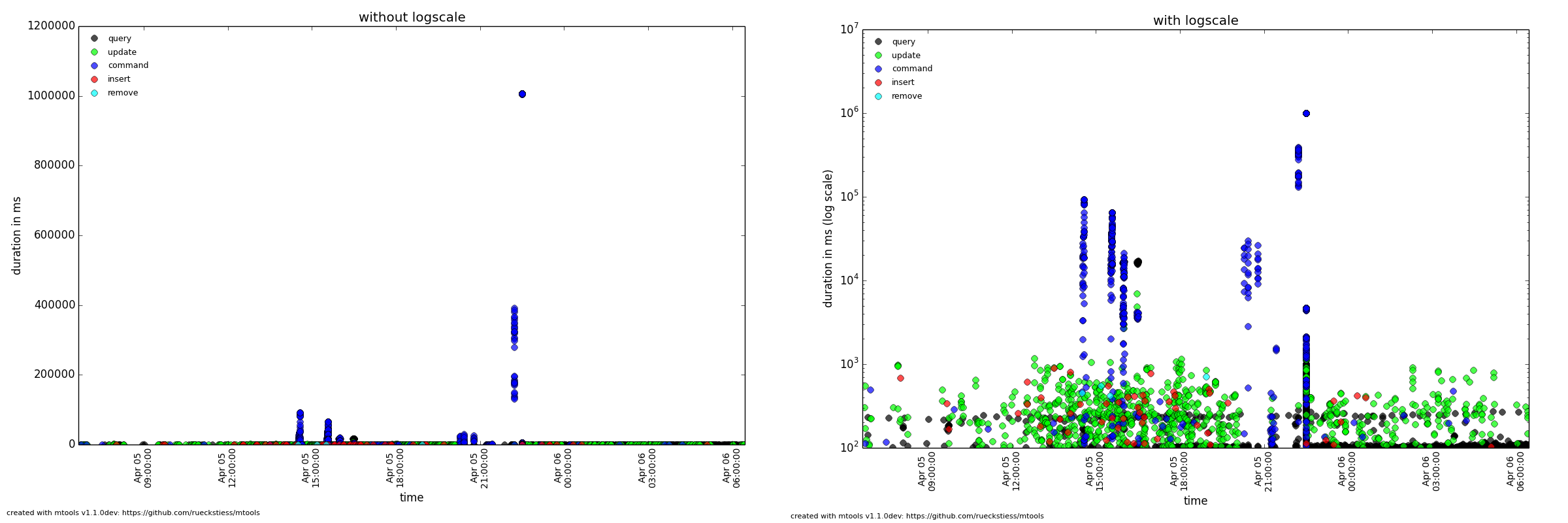
Logarithmic Scale#

--logscale: This option enables the logarithmic scale for plots where this makes sense. This is very useful if the plot contains outliers that squash all other data points to the bottom of the graph (see below comparison on the same data between log scale disabled and enabled). It can also be enabled with the l (lowercase L) shortcut once a plot is rendered. Switching scale on an already rendered plot may take a few seconds before the new scale is shown.

Custom Title#

--title: This option lets you overwrite the default title (the file name(s)) with a custom title. If the title contains spaces, the full title needs to be quoted in strings. The title of a plot is shown above the graph. A file read in from stdin does not use a title.

Operation Start Time#

--optime-start: Events are written to the log file when they finish, and by default, mplotqueries plots the operation on the x-axis at that point in time. Sometimes, it can be useful to see when operations started instead. For operations that have a duration (queries, updates, etc.) mplotqueries can subtract the duration and plot the operation when it started instead. Turn this feature on with the --optime-start flag.

Output to File#

--output-file: With this option, the plot can be written to a file rather than opening the interactive view window. The format is auto-recognized from the filename extension, with many supported formats, e.g. .png, .pdf, …

Checkpoints#

--checkpoints: This parameter enables information about slow checkpoints under WiredTiger, if available in the log files. The duration of checkpoints will be displayed in milliseconds. Terminal output will give an overview of the number of points to be plotted on the graph. The graph will contain the datetime and duration (in milliseconds) of slow checkpoints.

DNS#

--dns: Using this parameter slow DNS resolution can be identified and plotted. This flag will parse the log and collect available slow DNS information including hostname and time taken to resolve DNS. DNS information can be grouped by hostname using the --group flag.

OpLog#

--oplog: This parameter provides information about slow oplog operations. Output shows the number of slow operation detected in the log and the number of operations (points) plotted on the graph. The oplog will produce a scatter plot with respect to duration(milliseconds) and the date.

Groupings#

Group By#

--group GROUP

The group parameter specifies what the data should be grouped on. Grouping can have different meaning for the various plots below, but generally, groups are represented by color. A scatter plot would choose one color for each group. A histogram plot would also choose a color per group, but additionally stack the histogram groups on top of each other. Some plots don’t support grouping at all. See Plot Types for information about their grouping behavior.

The following values are possible for GROUP for most plots (some plots may not support all groups):

namespace (default for single file)
hostname
filename (default for multiple files)
operation (queries, inserts, updates, …)
thread
log2code (not supported by every plot type)
pattern (query pattern, e.g. {foo: 1, bar: 1}, no sub-documents)
custom grouping with regular expressions (see Python’s regex syntax)

For example:

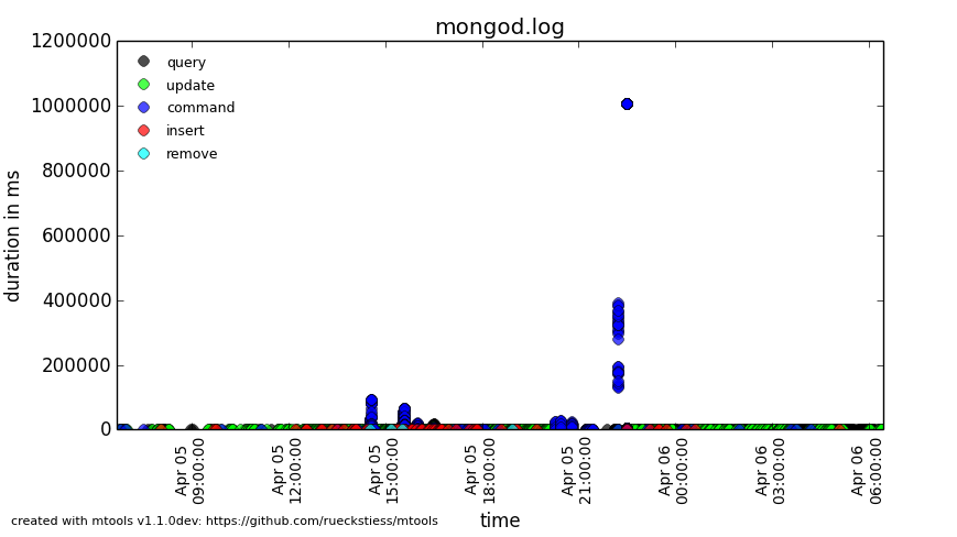
mplotqueries mongod.log --group operation

This command creates a scatter plot on duration (by default) and colors the operations (queries, inserts, updates, deletes, commands, getmores) in individual colors.

For example:

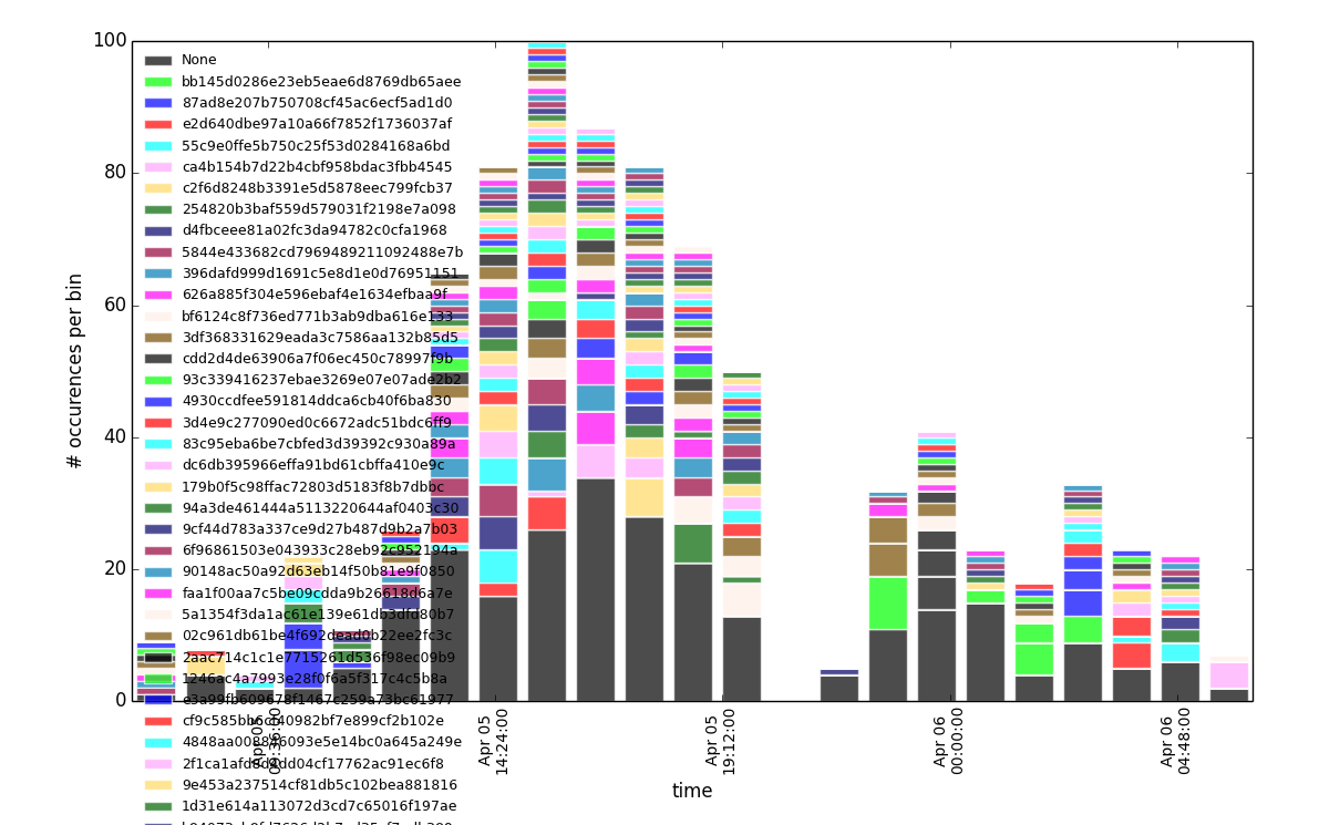
mlogfilter mongod.log --operation update --namespace test.users |
mplotqueries --type histogram --group "_id: ObjectId\('([^']+)'\)"

This command combination creates a histogram plot on duration of all the update operations on the test.users collection and groups the updates based on the _id ObjectId (extracted by the regular expression). If parentheses are present in the regular expression, then only the first matched group is being used as the group string (in this case, the 24 hex characters in the ObjectId). If parentheses are not present, the full regex match is being used as group string. Parentheses (and other reserved symbols) that need to be matched literally (like the parentheses in ObjectId('...') above) need to be escaped with a \.

If the number of groups is large, like in this example, it can be reduced with Group Limits.

Group Limits#

--group-limit N

This parameter will limit the number of groups to the top N, based on the number of matching lines per group (descending). The remaining groups are then grouped together in a single bucket called other. This option is useful if the number of groups is very large, as repetitions in color (there are only 14 distinct colors) could otherwise make it hard to distinguish all the groups for some plot types.

For example:

mplotqueries mongod.log --type range --group log2code --group-limit 10

This command creates a range plot, grouped on log2code, but only displays the 10 most frequently occurring log messages as separate groups. All others are plotted as one additional group others.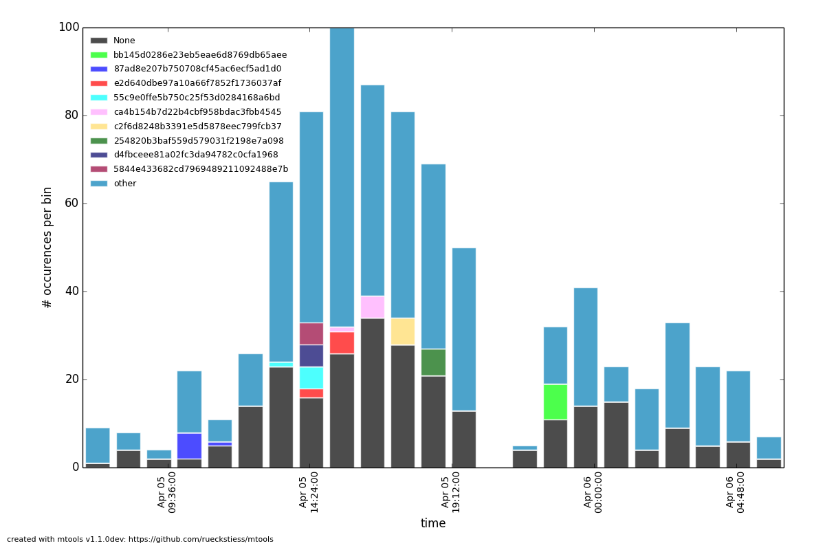

Plot Types#

Connection Churn Plot#

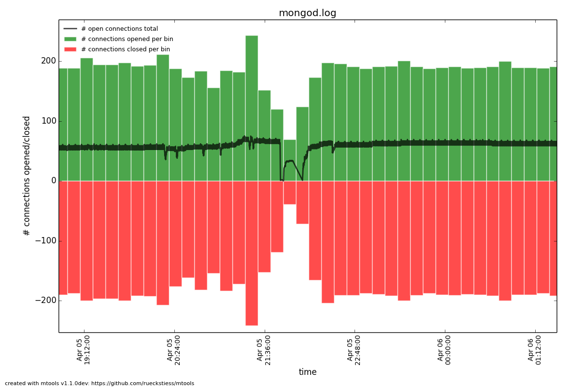
--type connchurn: A connection churn plot is a special plot that only considers lines about opening and closing connections. It will then create an opened (green bars) vs. closed (red bars) plot over time, and additionally show the number of currently open connections (black line, only for MongoDB log files >= 2.2).

Available Groupings#

No groupings are supported by this type of plot.

Additional Parameters#

--bucketsize SIZE, -b SIZE (alias)

As with histogram plots, this parameter sets the bucket size for an individual bucket (bar). The unit is measured in seconds and the default value is 60 seconds. This needs to be adjusted if the total time span of a log file is rather large. More than 1000 buckets are slow to render, and mplotqueries will output a warning to consider increasing the bucket size.

For example:

mplotqueries mongod.log --type connchurn --bucketsize 600

This command plots connection churn per 10 minutes (600 seconds) as a bi-directional histogram plot, as well as the total number of open connections at each time (black line).

Duration Line Plot#

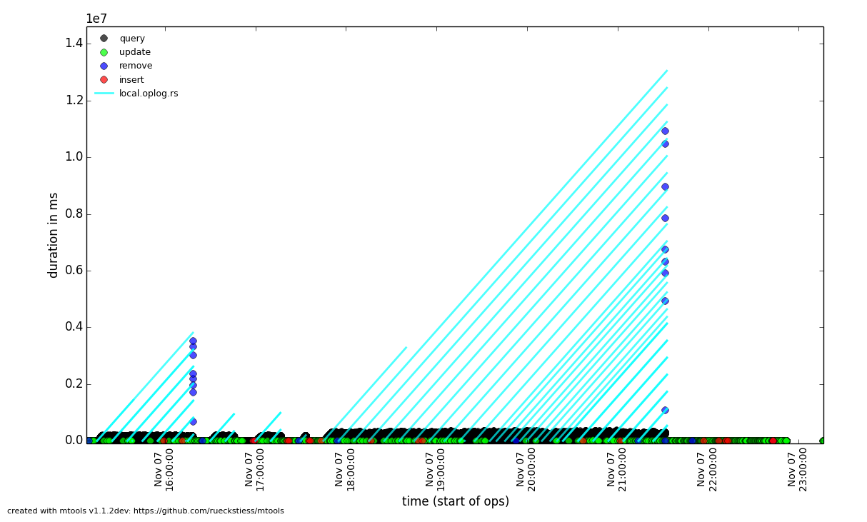
--type durline

The Duration Line plot shows operations that have a duration (like queries, updates, inserts, commands, etc). It draws a diagonal line from when the operation started (touching the x-axis) to when the operation stopped. This plot is especially useful to see when operations started and what impact they had on other queries during that time. It has the nice side-effect that all operations that started at the same time lie on the same diagonal line. Duration Line plots also make good plots to overlay with others.

For example:

grep "oplog.rs" mongod.log | mplotqueries --type durline --overlay
mplotqueries mongod.log --group operation

This command plots long-running oplog.rs operations as duration lines, and overlays them with a scatter plot of all operations.

Event Plot#

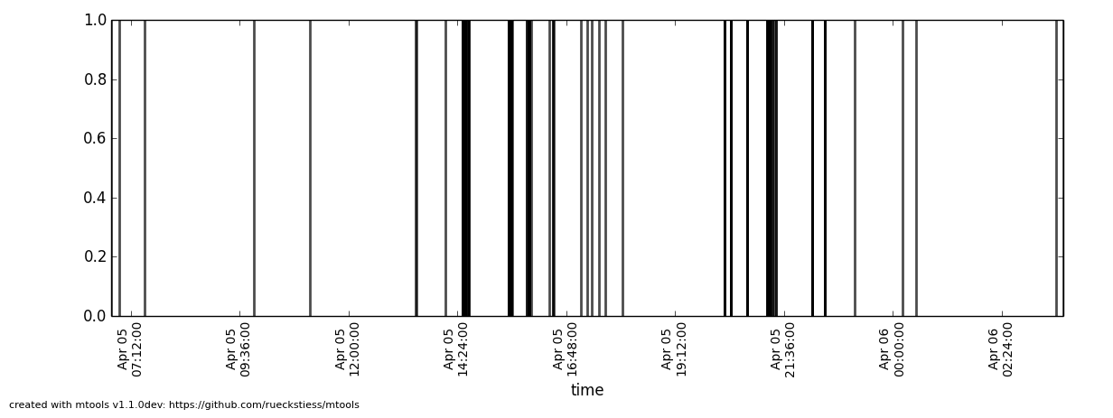
--type event

Event plots show the occurrence of certain events in a log file. They make sense mostly in combination with a preceding filter, either mlogfilter or a grep. For each matching event, a vertical line will be plotted at the time the event occurred. If the number of events is very large, you may want to consider using a range plot instead.

For example:

grep "getlasterror" mongod.log | mplotqueries --type event

This plot shows the occurrences of all “getlasterror” events in the log file.

Available Groupings#

Event plots use colors and to display different groups. The supported groupings for event plots are: namespace, operation, thread, filename (for multiple files), and regular expressions.

Additional Parameters#

No additional parameters are supported by this type of plot.

Histogram Plot#

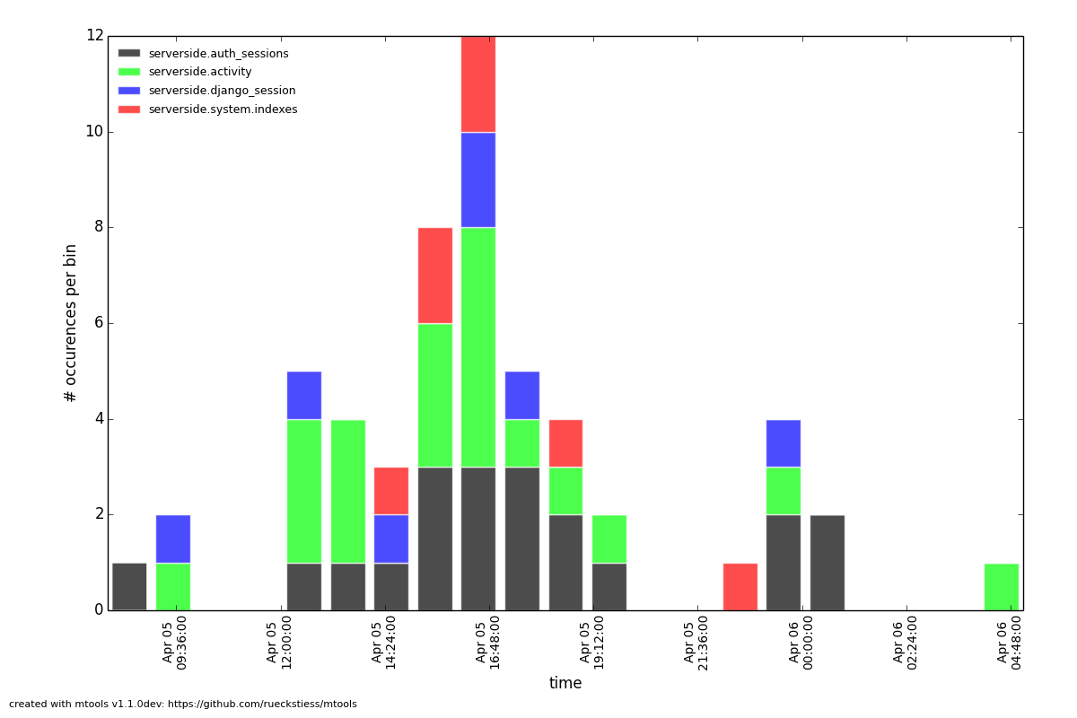
--type histogram: Histogram plots don’t consider a particular value in the log line (like for example scatter plots do), but rather bin the occurrence of log lines together in time buckets and present the result as a bar chart. The more occurrences of a certain log line (per group) in a given time frame, the higher the bar for that bucket. The size of a bucket is 60 seconds by default, but can be configured to another value (--bucketsize, see below). Unless one wants to know the total number of log lines per time bucket (which is not very useful information), this command should always be preceded with a filter, for example mlogfilter or grep.

Available Groupings#

Histogram plots use colors to display different groups. Each group gets its own bar, the bars are stacked on top of each other to also give an indication of the total number of matched lines per bucket. The supported groupings for histogram plots are: namespace, operation, thread, filename (for multiple files), log2code and regular expressions.

Additional Parameters#

--bucketsize SIZE, -b SIZE (alias)

This parameter sets the bucket size for an individual bucket (bar). The unit is measured in seconds and the default value is 60 seconds. This needs to be adjusted if the total time span of a log file is rather large. More than 1000 buckets are slow to render, and mplotqueries will output a warning to consider increasing the bucket size.

For example:

mlogfilter mongod.log --operation insert |
mplotqueries --type histogram --bucketsize 3600

This command plots the inserts per hour (3600 seconds) as a histogram plot. By default, the grouping is on namespace.

Example plot: histogram inserts per hour

Range Plot#

--type range: Range plots are good in displaying when certain events occurred and how long they lasted. For example, you can grep for a certain error message and use the range plot to see when these errors mostly occurred. For each group, a range plot shows one or several (if the --gap option is used) horizontal bars, that go from beginning to end of a certain event. If no --gap value is provided, the default is to not have any gaps at all, and the bar goes from the time of the first to the time of the last line of that group. If --gap is used, then the bar is interrupted whenever two consecutive log lines are further apart than the gap threshold.

Available Groupings#

Range plots use colors to display different groups. Each group gets its own horizontal bar(s). The supported groupings for range plots are: namespace, operation, thread, filename (for multiple files), log2code and regular expressions.

For example:

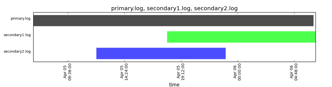
mplotqueries primary.log seconary1.log secondary2.log --type range

This plot shows for multiple files when they start and finish. By default, the grouping for multiple files is on filename, and as there is no gap threshold given, the bars range from the first two the last log line per file. This is useful to find out if and where several log files have an overlap.

Additional Parameters#

--gap LEN

If a gap threshold is provided, then the horizontal bars are interrupted when two consecutive events of the same group are further apart than LEN seconds.

For example:

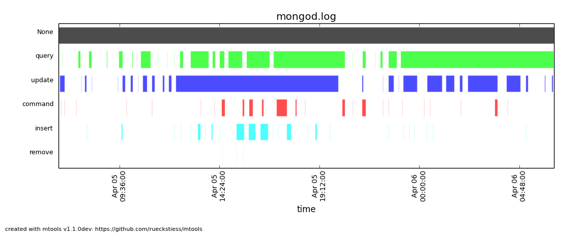
mplotqueries mongod.log --type range --group operation --gap 600

This plot shows ranges of contiguous blocks of updates where the gap threshold is 600 seconds (only gaps between two operations that are larger than 10 minutes are displayed as separate bars).

Replica Set State Plot#

--type rsstate

Replica set state plots are specialized event plots, that only consider lines about replica set state changes in a log file. They will display all changes of all replica set members (not just the node itself) with colored vertical lines, indicating different states. The most common states are PRIMARY, SECONDARY, ARBITER, STARTUP2, DOWN and RECOVERING, but other state changes are also displayed if found. This plot type helps to quickly determine any state changes at a given time. It is also useful to Overlays this plot with a different plot, for example a scatter plot.

For example:

mplotqueries mongod.log --type rsstate

This plot shows the state changes of all replica set members found in the log file.

Available Groupings#

No groupings are supported by this type of plot.

Additional Parameters#

No additional parameters are supported by this type of plot.

Scatter Plot#

--type scatter (default): A scatter plot prints a marker on a two-dimensional axis, where the x-axis represents date and time, and the y-axis represents a certain numeric value. The numeric value for the y-axis can be chosen with an additional parameter (--yaxis, see below). By default, scatter plots show the duration of operations (queries, updates, inserts, deletes, …) on the y-axis.

Available Groupings#

Scatter plots use colors and additionally different marker shapes (circles, squares, diamonds, …) to display different groups. The supported groupings for scatter plots are: namespace, operation, thread, filename (for multiple files), and regular expressions.

Additional Parameters#

--yaxis FIELD

This parameter determines what value should be considered for the location on the y-axis. By default, the y-axis plots duration. Other possibilities are nscanned, nupdated, ninserted, ntoreturn, nreturned, numYields, r (read lock), w (write lock).

For example:

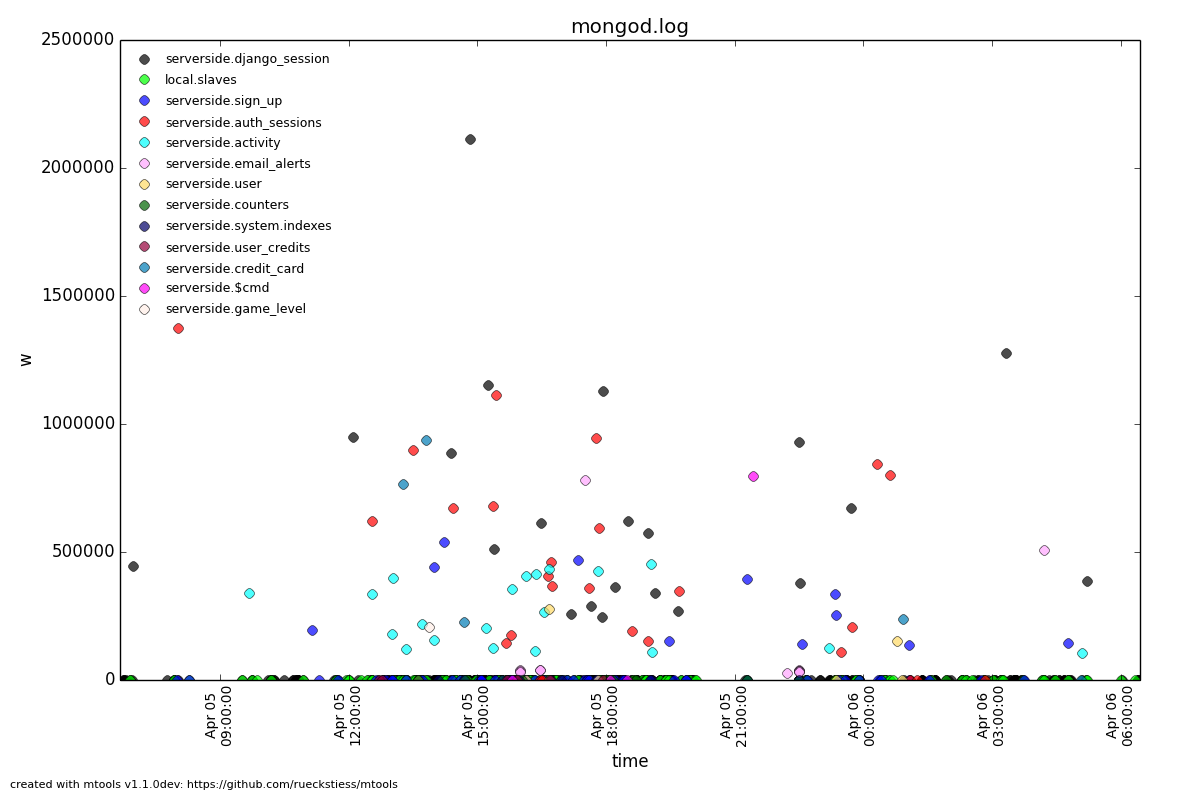
mplotqueries mongod.log --type scatter --yaxis w

This command plots the time (x-axis) vs. the write lock values of all operations (y-axis). Only lines that have a write lock value present are considered for the plot. Note that the unit for read/write lock is in microseconds.

--type nscanned

The scan ratio plot is a special type of scatter plot. Instead of plotting a single field as the standard scatter plot, it will calculate the ratio between the nscanned value and the nreturned value, and uses that result as the value for the y-axis. This plot is very useful to quickly find inefficient queries.

For example:

mplotqueries mongod.log --type nscanned/n

Overlays#

The overlay mechanism allows you to overlay several plot types in one graphic. This is useful to see correlations, match information from different plot types and create graphs that show events from different angles.

Each of the plot types can in theory be used as an overlay, however some of them make more sense then others.

Overlays are created just as normal plots, except they are stored on disk and do not render immediately. The first call to mplotqueries that does not add another overlay then will load all existing overlays added previously and render them on top of each other, matching the time axis.

Overlays are stored globally and are persistent, independent of your current working directory. Therefore, if you no longer need to store added overlays, make sure that you remove them again or they will be added to your next call of mplotqueries.

Plot types that are often used for overlays are: event, range, rsstate, and scatter.

Creating Overlays#

--overlay [add]: To create an overlay, run mplotqueries as you would normally, with all the command line arguments. In addition, specify the --overlay add argument. As add is the default for overlays, it can be omitted.

For example:

mplotqueries mongod.log --type scatter --overlay

Created overlay: 18124963

This will add an overlay plot. The plot is not shown but saved on disk instead, and rendered with the next call without --overlay.

List Existing Overlays#

--overlay list: To see if overlays are currently existing, you can use this command. A list of existing overlay identifiers will be returned. Currently, the indentifiers are not all that useful by themselves, but the command will show you how many different overlays exist.

Remove Overlays#

--overlay reset: To remove all overlays, you can use this command. It will delete all existing overlays, and the next (or current, if a log file is specified as well) call to mplotqueries will not show additional overlays.

Disclaimer#

This software is not supported by MongoDB, Inc. under any of their commercial support subscriptions or otherwise. Any usage of mtools is at your own risk. Bug reports, feature requests and questions can be posted in the Issues section on GitHub.